
Elliptical Orbits: Time-Dependent Solutions Using Kepler's Equation
The code KeplerEquation.m follows an orbiting body through one period of an elliptical orbit. It uses a series expansion involving Bessel functions to solve Kepler's equation.
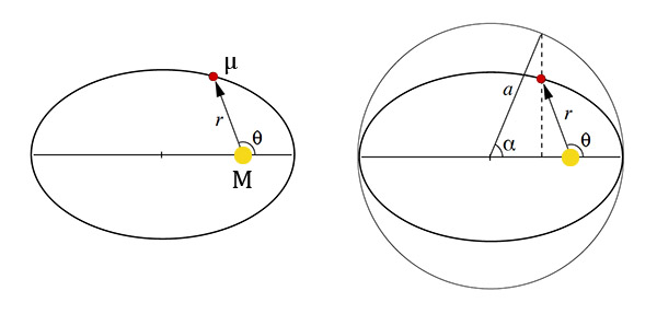
The left panel of the figure below shows a reduced-mass system in which an object with mass mu orbits a stationry object with mass M. The goal is to solve for the position of the orbiting object (in polar coordinates) aa a function of time.
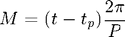
Johannes Kepler found the desired relationship in 1609 which is now called Kepler's Equation:

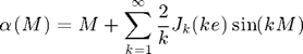
A series solution to Kepler's equation was provided by Bessel 1817. In fact, Bessel discovered his eponymous equations (the Bessel equations) as a means of solving Kepler's equation. He showed that solutions to Kepler's equations may be written as an infinite series of Bessel equations of the first kind:
Monkey Procedure:
To construct the positions of a planet as a function of time we follow this procedure:
- choose equally spaced values of the mean motion over one orbit, i.e. M will range from 0 to 2*pi
- for each value of M, use Bessel's solution to obtain the eccentric anomaly, alpha. One can try including different numbers of terms in the series solution to see how it affects accuracy.
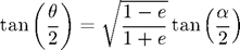
- calculate the true anomaly, theta, from the eccentric anomaly, alpha
- use the polar equation of an ellipse to calculate the radial coordinate, r, from the angle theta.
We now show the result and the code for an orbit with an eccentricity of 0.4 and a semi-major axis of 1.
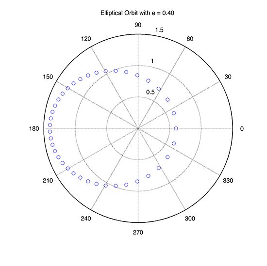
% KeplerEquation.m
%
% Follow an orbiting body through one period of an elliptical orbit
% Use Bessel's solution to Kepler's equation
%

clear           % clear variables
clc             % clear command window

e = 0.4;        % eccentricity
a = 1;          % semi-major axis
N = 40;         % number of points defining orbit

nTerms = 10;    % number of terms to keep in infinite series defining
                % eccentric anomaly

M = linspace(0,2*pi,N);   % mean anomaly parameterizes time
                          % M varies from 0 to 2*pi over one orbit

alpha = zeros(1,N);       % preallocate space for eccentric anomaly array


% Calculate eccentric anomaly at each point in orbit
for j = 1:N
    % initialize eccentric anomaly to mean anomaly
    alpha(j) = M(j);

    % include first nTerms in infinite series
    for n = 1:nTerms
        alpha(j) = alpha(j) + 2 / n * besselj(n,n*e) .* sin(n*M(j));
    end
end

% calcualte polar coordiantes (theta, r) from eccentric anomaly
theta = 2 * atan(sqrt((1+e)/(1-e)) * tan(alpha/2));
r = a * (1-e^2) ./ (1 + e*cos(theta));

% polar plot of orbit
polar(theta,r,'bo');

% Label plot with eccentricity
title(['Elliptical Orbit with e = ' sprintf('%.2f',e)]);

% Save plot as pdf
set(gcf, 'PaperPosition', [0 2 8 8]);
print ('-dpdf','kepler.pdf');
Monkey Commentary:
The code is fairly straightforward. The only thing that might be new is the Bessel function found on this line:
alpha(j) = alpha(j) + 2 / n * besselj(n,n*e) .* sin(n*M(j));
The function besselj(k,x) returns the kth Bessel function of the first kind evaulated at x.