plot09.m - Parametric Plot Example: Lissajous Figures

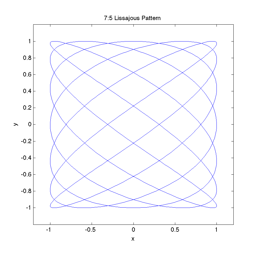
kx = 7;      % wavenumber of x wave
ky = 5;      % wavenumber of y wave

t = linspace(0,2*pi,1000);  % define 1000 x values from 0 to 2 pi

x = sin(kx*t);               % x wave
y = sin(ky*t+pi/2);          % y wave

plot(x,y,'b-')              % plot blue curve
axis equal                  % scale same for both axes
axis([-1.2 1.2 -1.2 1.2]);  % set plot range

% label axes and add title
xlabel('x');
ylabel('y');
str = sprintf('%i:%i Lissajous Pattern',kx,ky);
title(str);

Download plot09.m

Parametric plots use a parameter (say t) to calculate the the x and y coordinates (x(t), y(t)). Lissajous figures are easily written in parametric form as: $$x(t) = \sin(k_x t)$

$y(t) = \sin(k_y t + \phi_0)$

The figures form closed curves when the wavenumbers $k_x$ and $k_y$ are commensurable, i.e. $k_x/k_y$ is a rational number.

Notice the use of the axis equal command. This ensures that the scaling is the same for the x and y axes. Thus, a circle will appear as a circle rather than an ellipse.

Monkey Home | Prev | Next